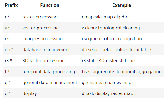
Using GRASS GIS in Jupyter Notebooks:
An Introduction to grass.jupyter

Caitlin Haedrich, Vaclav Petras, Anna Petrasova

NCSU GeoForAll Lab at the Center for Geospatial Analytics
North Carolina State University

Caitlin Haedrich

• PhD student GeoForAll Lab at North Carolina State University
• Advised by Helena Mitasova (and Anna Petrasova and Vashek Petras)
• Interested in geovisualization and increasing accessibilty of GIS tools
• Working with integrating GRASS GIS with Jupyter through Google Summer of Code 2021 and Mini Project Grant from GRASS GIS
• TA for graduate-level Geospatial Computation and Simulation

Teaching Geospatial Analytics

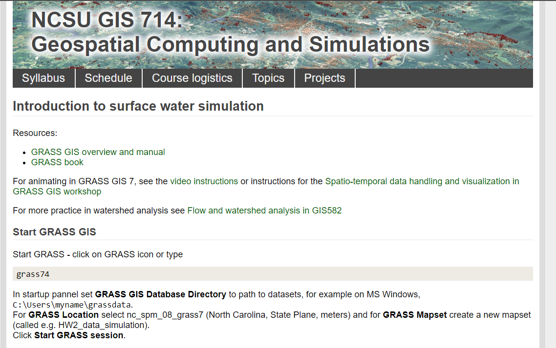
GIS714: geospatial computation and simulation

Graduate level course required for Geospatial Analytics PhD students

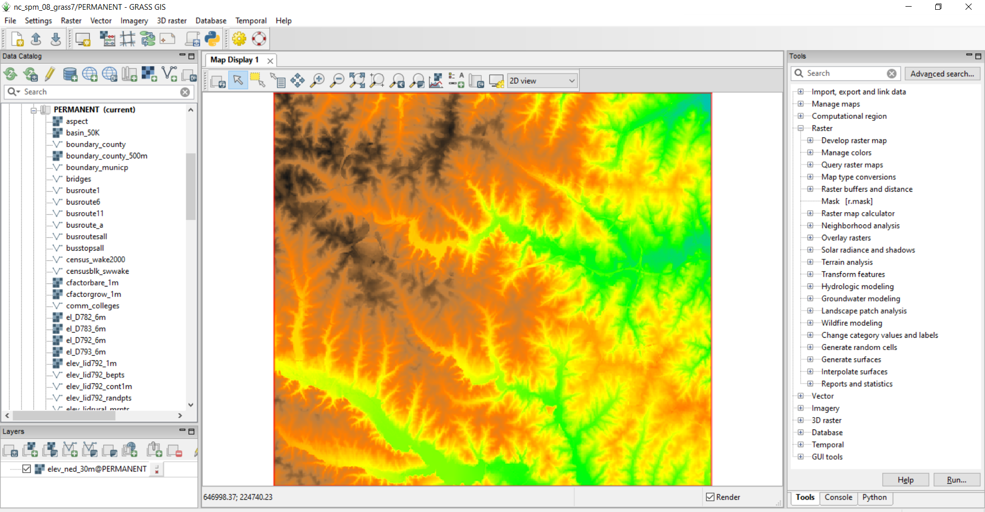
Previously taught with GRASS tutorials, instructions posted on webpage

Goal: convert to GRASS-based assignments in Jupyter Notebooks

GRASS GIS

• Open-source GIS software with over 500 tools and 400 addons
• Interfaces: graphical user interface, command line, Python, C
• 3rd Party Interfaces: R, QGIS, actinia (REST API)

Project Jupyter

“The Jupyter Notebook is an open-source web application that allows you to create and share documents that contain live code, equations, visualizations and narrative text.” – jupyter.org

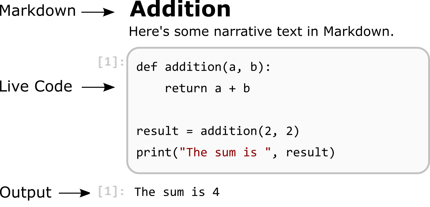
The default kernel is IPython.

import sys

v = sys.version_info
print(f"We are using Python {v.major}.{v.minor}.{v.micro}")

We are using Python 3.9.5

Output can be interactive.

from ipywidgets import interact

def f(x):
    return x

interact(f, x=10);

grass.jupyter

...enhances the existing GRASS Python API to allow Jupyter Notebook users to easily manage GRASS data, visualize data including spatio-temporal datasets and 3D visualizations

• Released with main GRASS GIS distribution starting in version 8.2
• Python package that makes GRASS more accessible in Jupyter by providing:
  • Data management functions
  • Visualizations classes for viewing and interacting with GRASS through in-line figures
• Created with syntax consistent with GRASS's existing Python API and command line interface

You can also try it out in Binder:

Teaching Geospatial Computation and Simulation with grass.jupyter

GIS714: Geospatial Computation and Simulation, Spring 2022

Course Repo on GitHub

We'll use an example from the course on water simulation...

Getting Started

# Import Python standard library and IPython packages we need.
import subprocess
import sys

# Ask GRASS GIS where its Python packages are.
sys.path.append(
    subprocess.check_output(["grass80", "--config", "python_path"],
                            text=True, shell=True).strip()
)

# Import the GRASS GIS packages we need.
import grass.script as gs
import grass.jupyter as gj

# Start GRASS Session
session = gj.init("data", "nc_spm_08_grass7", "HW3_water_simulation")

# Set region to the high resolution study area
gs.run_command("g.region", region="rural_1m")

gj.init starts session, sets GRASS environmental variables for notebooks

And then we are ready to begin using GRASS!

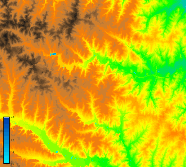
Create a map of flooded area

We create a map of flooded area with r.lake (GRASS manual for r.lake) by providing a water level and a seed point:

gs.run_command("r.lake", elevation="elev_lid792_1m", water_level=113.5,
               lake="flood1", coordinates="638728,220278")

# See results
flood1 = gj.Map(use_region=True, width=200)
flood1.d_rast(map="elev_lid792_1m")
flood1.d_rast(map="flood1")
# Display map
flood1.show()

Question 4

Increase water level to 113.7m and 114.0m and create flooded area maps at these two levels.

#### Your Answer Here

We can also make 3D maps using similar syntax

elev_map = gj.Map3D()
elev_map.render(elevation_map="elevation", color_map="elevation",
                perspective=20)
elev_map.overlay.d_legend(raster="elevation", at=(60, 97, 87, 92))
elev_map.show()

Syntax: Integrating GRASS Display Modules with grass.jupyter

We can call display modules using Python magic short-cut (__getattr__):

To add a raster, we need d.rast so we use Map.d_rast(), Map3D.overlay.d_rast

Estimating inundation extent using HAND methodology

We will use two GRASS addons, r.stream.distance and r.lake.series, to estimate inundation with Height Above Nearest Drainage methodology (A.D. Nobre, 2011).

For this section, we will change our computation region to elevation which is a larger study area than we used above. We use r.watershed to compute the flow accumulation, drainage and streams.

gs.run_command("g.region", raster="elevation")
gs.run_command("r.watershed", elevation="elevation", accumulation="flowacc",
               drainage="drainage", stream="streams_100k", threshold=100000)
gs.run_command("r.to.vect", input="streams_100k", output="streams_100k",
               type="line")

Now we use r.stream.distance with output parameter difference to compute new raster where each cell is the elevation difference between the cell and the the cell on the stream where the cell drains. This is our HAND terrain model.

gs.run_command("r.stream.distance", stream_rast="streams_100k",
               direction="drainage", elevation="elevation",
               method="downstream", difference="above_stream")

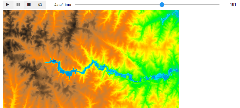
With r.lake.series, we can create a series of inundation maps with rising water levels. r.lake.series creates a space-time dataset. We can use temporal modules to further work with the data...

gs.run_command("r.lake.series", elevation="above_stream",
               start_water_level=0, end_water_level=5, water_level_step=0.5, 
               output="inundation", seed_raster="streams_100k")

... or visualize the flood with TimeSeriesMap.

flood_map = gj.TimeSeriesMap(use_region=True)
flood_map.d_rast(map="elevation")
flood_map.add_raster_series("inundation")
flood_map.d_legend(color="black", at=(2,30,2,5)) #Add legend
flood_map.show()

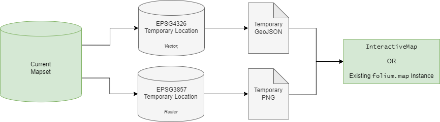
folium Integration for Interactive Maps

Interactivity is often useful for explore geospatial data.

folium...

• is a popular Python library for creating Leaflet.js maps

• creates interactive HTML maps that can be displayed in-line

• has built-in tilesets from OpenStreetMap, Mapbox, and Stamen, and supports custom tilesets

Moving data from GRASS GIS location projection to folium is a challenge

folium is projected in Web Mercator (EPSG:3857)

However, any coordinates (i.e. vector data) need to be specified in degrees of latitude and longitude (WGS84, EPSG:4326)

We pass data to folium by reprojecting to temporary locations

import folium 

# Create figure
fig = folium.Figure(width=600, height=400)

# Create a map to add to the figure later
m = folium.Map(tiles="Stamen Terrain", location=[35.761168,-78.668271],
               zoom_start=13)

# Create and add elevation layer to map
gj.Raster("elevation", opacity=0.5).add_to(m)

# make a tooltip
tooltip = "Click me!"
# and add a marker
folium.Marker(
    [35.781608,-78.675800],
    popup="<i>Center For Geospatial Analytics</i>",
    tooltip=tooltip
).add_to(m)

# and a circle
folium.Circle(
    radius=120,
    location=[35.769781,-78.663160],
    popup="Great Picnic Area",
    color="crimson",
    fill=False,
    tooltip=tooltip
).add_to(m)

# Add the map to the figure
fig.add_child(m)

# Display figure
fig

The InteractiveMap class allows users unfamiliar with folium to produce maps easily.

# Create Interactive Map
fig = gj.InteractiveMap(width = 600)
# Add raster, vector and layer control to map
fig.add_raster("elevation", title="Elevation Raster", opacity=0.8)
#fig.add_vector("roadsmajor")
fig.add_layer_control(position = "bottomright")
# Display map
fig.show()

Course Reflections

Notebook format was generally well received:

• Several students noted they enjoyed being able to experiment with GRASS tools by varying parameters and visually observing the effect.
• GitHub and Binder allowed students to easily access and run the notebooks
  • This also gave the students exposure to working with Git and GitHub, an important tool for open science and collaborative research.

We did experience some challenges:

• Running the notebooks locally was difficult for many students.
• Students running notebooks locally often encountered issues that were OS or GRASS version-specific issues.
• Binder occasionally unreliable.
• Prerequisites include having basic Python skil, familiarity with the fundamentals of geospatial analysis and some experience using Jupyter Notebooks.

grass.jupyter

Session Management

Visualization Methods: Map, Map3D, TimeSeriesMap, folium-integration and InteractiveMap

Future Work

• improved formatting of text output from GRASS tools
• add a raster legend to InteractiveMap and GRASS-folium maps.
• current implementation of InteractiveMap cannot display large images; offering a tiling method using gdal tools could be a solution.
• TimeSeriesMap is also quite time-consuming; rendering time could be further reduced by parallelizing the raster rendering.
• ipyleaflet as alternative to folium

More Resources

grass.jupyter Manual Page

FOSS4G '22 GRASS GIS Workshop Materials (Anna Petrasova)

GIS714: Advanced Geospatial Computation and Simulation Course Repository

Example Notebooks in GRASS GIS's GitHub Repository (can be run with binder through link provided in main repo README)

Link to these slides

Thank you to...

Helena Mitasova

Stefan Blumentrath

Vero Andreo

GIS714 Class Spring 2021

… and the GRASS community, NC State Center for Geospatial Analytics, Google Summer of Code